Image Preparation

Regardless of training location or modality, both training and inference require consistent image preparation and preprocessing. In these sections, we describe some important aspects of preprocessing that you may want to include in your training and inference workflows, including:

• Bit depth, or how much information is included in a single pixel in an image

• Histogram image transformations that can be used to enhance the quality of an image and/or alter an image’s bit depth

• Image chipping, or how to take a single image with many pixels and transform it into many images with fewer pixels

Bit Depth

Bit depth refers to the granularity of colors that can be stored in a single pixel of an image. Though this is not a perfect analogy, it is helpful to think of this number as the amount of information that can be stored in a single pixel.

Common consumer imagery (like that from a digital camera like a smartphone) is typically 8-bit color imagery. The fact that the imagery is color means that each pixel will have more than one (color) channel; there are usually three channels: red (R), green (G), and blue (B), or RGB. Any pixel's value (or color) is described by three numbers: a number for the red intensity, a number for the green intensity, and a number for the blue intensity. Bit depth is the number of bits used to encode these intensity numbers.

An 8-bit image will use 8 bits to encode the intensity in each color channel. You can use 8 bits to describe a total of 2^8 = 256 different values (for each channel). Therefore, the intensity for each channel in an 8-bit image is an integer between 0 (dark, minimum intensity) and 255 (bright, maximum intensity).

Determining the Bit Depth of an Image

There are several ways to determine the bit depth of an image. Which method you use depends on the file type (e.g., PNG, JPEG, NITF, etc.), your available tools, and your willingness and ability to write code.

Method 0: JPEG Files Are All 8-Bit

If you have a JPEG file (either .jpeg, .jpg, or .jfif file extension), the image is an 8-bit image. The JPEG standard only supports 8-bit imagery.

NOTE: Renaming a file does not change its contents. So, if, for example, you rename my_file.nitf to my_file.jpeg, that does not create a JPEG file for you; it is still a NITF file. So, looking at the file extension to determine that you have an 8-bit image is not always sufficient.

Method 1: Using the Bash file utility

Open a terminal and run:

$ file /path/to/my/image.png

Depending on the file type, you may see various outputs. Below are example outputs with explanations.

• PNG file (example 1)
  /path/to/my/image.png: PNG image data, 600 x 600, 8-bit/color RGBA, non-interlaced
  The PNG image data confirms that this is a PNG image.
  The 8-bit/color RGBA tells us this is an 8-bit image with four channels: red, green, blue, and alpha (transparency).

• PNG file (example 2)
  /path/to/my/other/image.png: PNG image data, 852 x 724, 16-bit grayscale, non-interlaced This image is also a PNG but is 16-bit and has a single channel (grayscale).

• JPEG file
  /path/to/my/jpg/image.jpg: JPEG image data, JFIF standard 1.01, aspect ratio, density 1x1, segment length 16, baseline, precision 8, 183x275, components 3
  The JPEG image data confirms that this image is a JPEG—and we know it is 8-bit. In addition, the precision 8 confirms that this is an 8-bit image.
  The components 3 indicates that this is a color image with three channels: red, green, and blue.

• NITF file
  /path/to/my/nitf/image.nitf: National Imagery Transmission Format dated 20190105095921
  This method is unlikely to work for NITF files; unfortunately, it only confirms that the format is indeed NITF.

Method 2: Using the Bash exiftool utility

This tool parses some of the EXIF metadata associated with an image. It provides much greater detail than the file utility, though it is less likely to be installed by default and may require elevated privileges to install.

This tool may not work with all NITF files. It is likely to work with NITF-encoded GeoTIFFs but is unlikely to work with other NITF files.

To run the tool (if installed), open a terminal and run:

$ exiftool /path/to/my/image.png

Depending on the file type and available metadata, you may see a variety of different outputs, as in the following example:

ExifTool Version Number         : 11.88
File Name                       : image.png
Directory                       : /path/to/my
File Size                       : 40 kB
File Modification Date/Time     : 2023:07:11 11:13:51-05:00
File Access Date/Time           : 2023:08:22 10:28:28-05:00
File Inode Change Date/Time     : 2023:07:11 11:13:51-05:00
File Permissions                : rw-r--r--
File Type                       : PNG
File Type Extension             : png
MIME Type                       : image/png
Image Width                     : 600
Image Height                    : 600
Bit Depth                       : 8
Color Type                      : RGB with Alpha
Compression                     : Deflate/Inflate
Filter                          : Adaptive
Interlace                       : Noninterlaced
Pixels Per Unit X               : 3937
Pixels Per Unit Y               : 3937
Pixel Units                     : meters
Image Size                      : 600x600
Megapixels                      : 0.360

As you can see, the output contains significantly more information about the image than the first method. The exact information will depend on the image, the metadata present, and the metadata parseable by ExifTool.

In this example, the relevant information is the bit depth, which we see is 8, so we know this is an 8-bit image. Note that the name of the metadata field may change from data type to data type. For example, the field may be called “bits per sample” in a TIFF or GeoTIFF file.

Method 3: Python Code with Rasterio

While this method won’t give you all the metadata (e.g., precisely what your bit depth is), it can quickly tell you whether or not your image is 8-bit or not.

Open a Python shell and run the following commands:

>>> import rasterio
>>> src = rasterio.open("/path/to/img.nitf")
>>> arr = src.read(1)
>>> src.close()
>>> print(arr.dtype)

The most likely things you will see for the arr.dtype (array’s data type) are either uint8 or uint16, though other options are possible. If you see anything other than uint8, your image is almost certainly not 8-bit.

Why does the bit-depth of my imagery matter?

Why Bit Depth Matters

Chariot’s training and inference services currently rely on the Python Imaging Library (PIL) for various image transforms. Those image transforms include image resizing and all the data augmentations used during training. Because Chariot depends on PIL for these transforms, we can only use PIL-supported types internally for training, and those are (with very few exceptions) limited to 8-bit types.

In the sections that follow, we describe several methods that can be used to create PIL-supported 8-bit imagery.

We note that Chariot now provides a mechanism for applying the recommended options below to imagery during training at a user’s discretion.

The documentation and code below provide the following:

• Understanding for the user of what happens under the hood
• The ability to implement one’s own preprocessing pipeline (to maintain full control)
• The ability to improve performance (training speed) by preprocessing the imagery once (before upload) instead of preprocessing it every time a datum is seen
• The ability to ensure that the same preprocessing that happens during training is applied for inference

Image Preprocessing

There are various ways to preprocess imagery and various goals that can be achieved. In this section, we primarily focus on producing 8-bit imagery. However, many of these techniques can also be applied to improve image perception by human eyes, possibly also impacting a model’s perception.

The most critical aspect of preprocessing is that once a model is trained, the process should be the same for training and production data. Preprocessing can impact the data distribution; if the preprocessing pipeline differs from training to production, model inference quality will almost certainly suffer.

Method 1: Naive Rounding (Not Recommended)

While not recommended, the simplest method is rounding. This method is rarely useful because pixel values tend to be concentrated in a small range of possible values. If we round over the entire range evenly, information is lost needlessly. However, this method can be useful if the image’s histogram is uniform throughout its range.

At a high level, you find the largest value: either 2^(bit depth) - 1, or the largest observed pixel value in the image (especially if the exact bit depth is unknown). If all the pixel values are divided by this largest number, the result will be in the range of [0, 1]. Then, multiply all the values by 255 so that you are in the range of [0, 255], and round to the nearest integer.

Following that procedure, the minimum pixel values will typically not reach 0; there is an unused range of values. To use the full range of values, you could first subtract the smallest observed pixel value from every pixel. Then, follow the procedure above (dividing by a maximum value, multiplying by 255, and rounding).

The following code accomplishes this.

import rasterio
import numpy as np
from PIL import Image

src = rasterio.open("/path/to/image.nitf")
arr = src.read(1)
src.close()

# Shift all values down so that the smallest pixel value is 0.
min_value = np.min(arr)
arr = arr - min_value

# Divide by maximum value (pushes all pixels into [0, 1] range)
max_value = np.max(arr)
arr = arr / max_value

# Scale up and round
arr = (255 * arr).astype("uint8")

# Save the preprocessed image for upload in a Chariot dataset.
# Note: PIL will save this file in the type specified by the suffix (in this case PNG).
Image.fromarray(arr).save("/path/to/new/image.png")

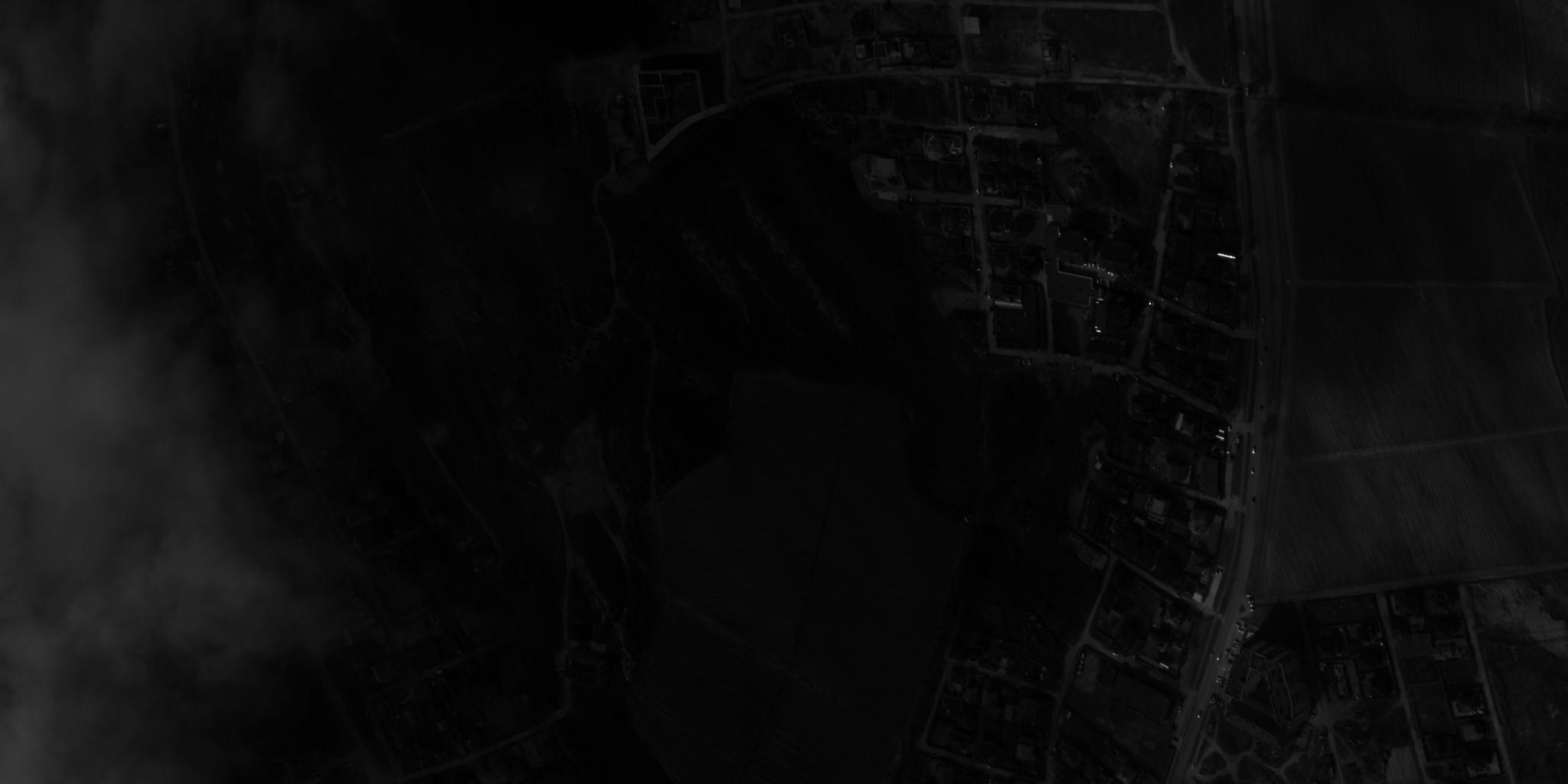
Below (Figure 1) is an example image. The source was an 11-bit NITF file, which resulted in a naively stretched, 8-bit JPEG image.

Figure 1: A sample 11-bit NITF image naively rounded to an 8-bit JPEG image

Method 2: Linear Stretching (Recommended)

Linear stretching follows the same idea as above: Subtract a minimum value, divide by the maximum value, scale back up, and round. The difference is which values get treated as the minimum and maximum values. For example, we will pick a “minimum” value to subtract that is not the actual minimum pixel value, and we will pick a “maximum” value to divide by that is not the actual maximum pixel value.

Figure 2: The histogram of pixel intensities for the sample 11-bit NITF image

The problem with the naive method is that there tends to be a long, narrow tail on the distribution of pixel intensities (see Figure 2). This histogram represents the counts of various pixel intensities in the raw NITF file that was used to produce the naively rounded JPEG in Method 1 above. The maximum pixel value in that image is, in fact, at the extreme right of that plot—the frequency is just too small to see. So, when we squish all those values into the 0–255 range, we only effectively use 10–20% of the possible pixel values. As a result, the image’s color is very evenly dark, and features are hard to see. If we choose a maximum value closer to 500 and a minimum value closer to 200, we will effectively use all the available intensities.

If we want to make a 2% stretch, we will find two values: the 2nd percentile of pixel values and the 98th percentile of pixel values. We will then call anything over the 98th percentile “fully saturated” (maximum value), and we will call any values under the 2nd percentile “fully dark” (minimum value).

In code, that looks like the following:

import rasterio
import numpy as np
from PIL import Image

src = rasterio.open("/path/to/image.nitf")
arr = src.read(1)
src.close()

# Find the 2nd and 98th percentile values
lower, upper = np.percentile(arr.flatten(), [2, 98])

# Subtract the minimum, divide by the (adjusted) maximum.
arr = (arr - lower)/(upper - lower)

# Clip the array so that anything below 0 becomes 0 and anything above 1 becomes 1.
arr = np.clip(arr, a_min=0, a_max=1)

# Scale to 255 and round.
arr = (arr * 255).astype("uint8")

# Save the preprocessed image for upload in a Chariot dataset.
Image.fromarray(arr).save("/path/to/new/image.png")

This method is flexible; the 2% stretch was a choice. We could experiment with other values (e.g., a 3% stretch, a 5% stretch, etc). The important thing is that whatever we choose, we consistently use it for training and inference.

Below (Figure 3) is the same example image as above but with a 2% linear stretch applied.

Figure 3: A sample 11-bit NITF image with a 2% linear stretch applied

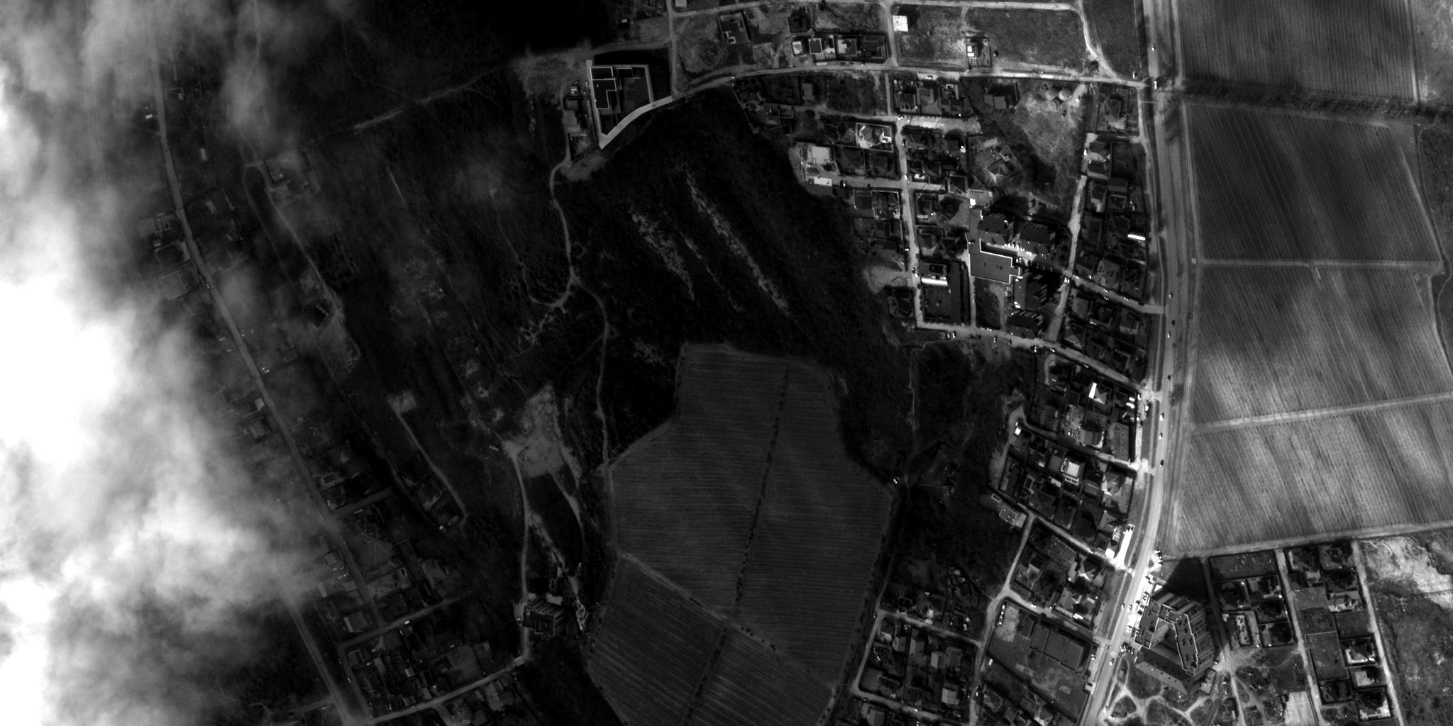
If we examine the resulting histogram (Figure 4), we can now easily see that we have used the full range of possible pixel values. However, there is still a heavy tail on the lower end, which reflects the large portion of the image (center) that appears darker than average.

Figure 4: The histogram of pixel intensities of the sample NITF image after a 2% linear stretch was applied

Method 3: Contrast Limited Adaptive Histogram Equalization (Recommended)

While linear stretching tends to be an improvement over naive rounding, the shape of the histogram can still be skewed. Contrast-limited adaptive histogram equalization (CLAHE) is a process similar to a linear stretch, except that the amount of adjusted pixels is not constant. Pixels are binned in a fashion that attempts to equalize the histogram.

In this code example, we use the implementation equalize_adapthist from the scikit-image. There is one required parameter in this method, nbins. Since we are creating 8-bit imagery, we need nbins=256 (2^8). Note that this method is agnostic to the bit depth of the original image.

import rasterio
import numpy as np
from PIL import Image
from skimage import exposure

src = rasterio.open("/path/to/image.nitf")
arr = src.read(1)
src.close()

# Creates an array of pixel values in the [0, 1] range taking on 256 different values.
arr = exposure.equalize_adapthist(arr, nbins=256)

# Scale to [0, 255] and round to nearest integer.
arr = (arr * 255).astype("uint8")

# Save the preprocessed image for upload in a Chariot dataset.
Image.fromarray(arr).save("/path/to/new/image.png")

As illustrated above, our original example image, with CLAHE preprocessing applied, yields the following image.

Figure 5: Sample 11-bit NITF image with CLAHE preprocessing applied

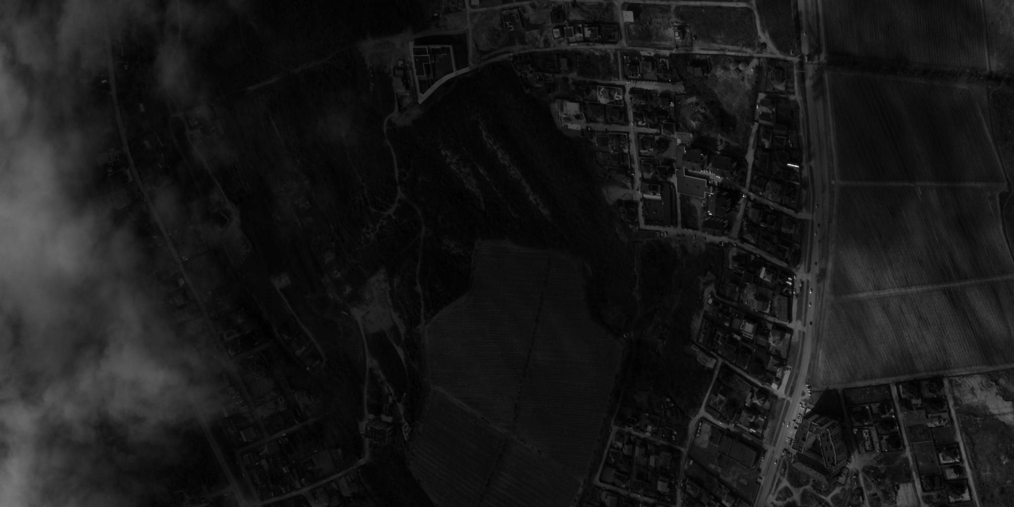
The goal of CLAHE is to approximately equalize the histogram. The resulting histogram is below (Figure 6); in this case, CLAHE failed to approximately equalize the histogram because of the extreme outliers. It is debatable whether this method or the linear stretch alone was better.

Figure 6: The histogram of pixel intensities of the sample 11-bit NITF image preprocessed with CLAHE

The effectiveness of linear stretch or CLAHE depends on the characteristics of the original image. Regardless of which preprocessing method(s) you choose, it is critical to maintain consistency between training data and production data.

Method 4: CLAHE and Linear Stretching (Recommended)

One often effective method is applying both CLAHE and linear stretch. Below, we illustrate how to do this by applying linear stretch first; the two methods can be applied in any order, and your chosen order creates different results.

import rasterio
import numpy as np
from PIL import Image
from skimage import exposure

src = rasterio.open("/path/to/image.nitf")
arr = src.read(1)
src.close()

# Make the 2% linear stretch exactly as before.
lower, upper = np.percentile(arr.flatten(), [2, 98])
arr = (arr - lower)/(upper - lower)
arr = np.clip(arr, a_min=0, a_max=1)

# Apply CLAHE
arr = exposure.equalize_adapthist(arr, nbins=256)

# Scale and round
arr = (arr * 255).astype("uint8")

# Save the preprocessed image for upload in a Chariot dataset.
Image.fromarray(arr).save("/path/to/new/image.png")

The following is the resulting example image.

Figure 7: Sample 11-bit NITF image with a 2% linear stretch and CLAHE applied

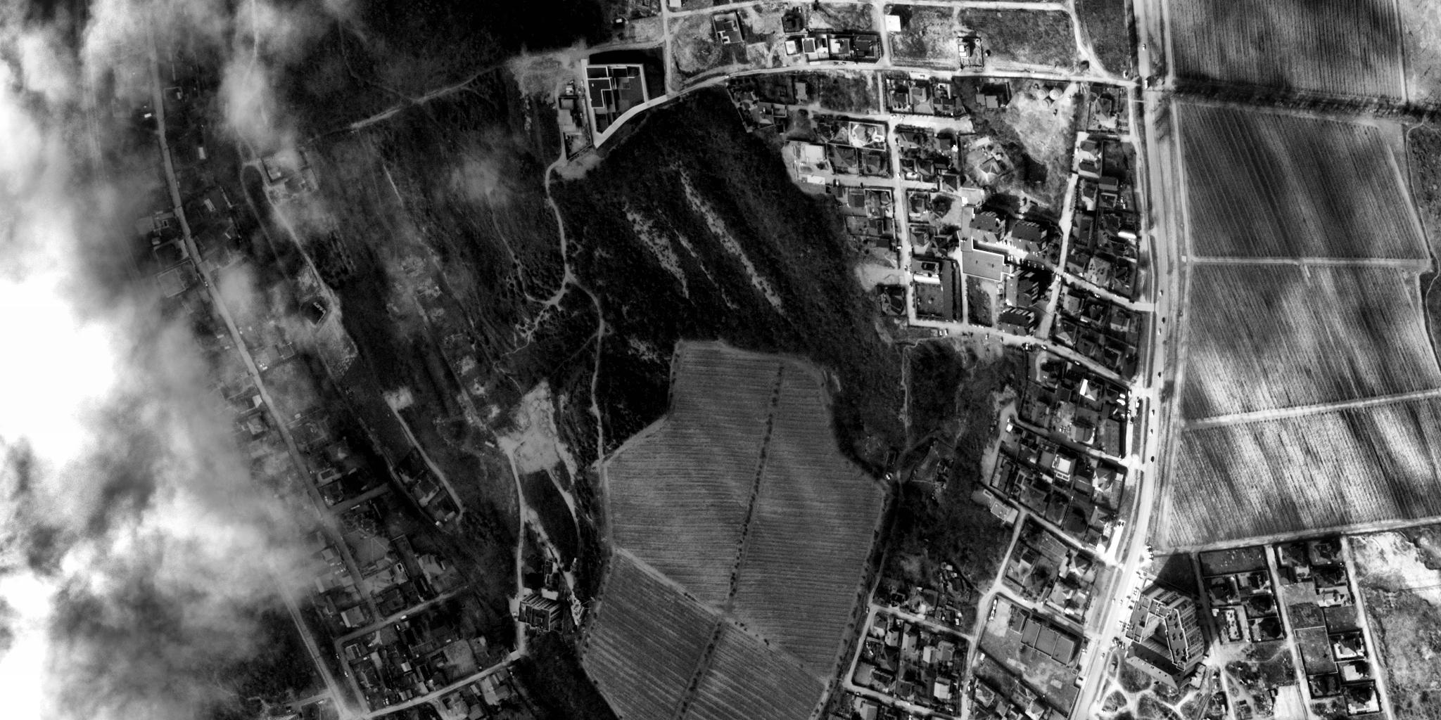
And, as you might expect from the quality of the image, the histogram is significantly closer to equal.

Figure 8: The histogram of pixel intensities of the sample 11-bit NITF image with a 2% linear stretch and CLAHE applied

Image Chipping

The biggest question here is whether you should chip and then apply preprocessing (in one of the forms above) or apply the preprocessing globally and then chip the result.

While both methods are acceptable, if you apply one of the recommended forms of preprocessing after chipping, you will have more consistent image characteristics and a more consistent data distribution, which generally helps model performance. We therefore recommend chipping the data and then applying the preprocessing method above to each chip independently.

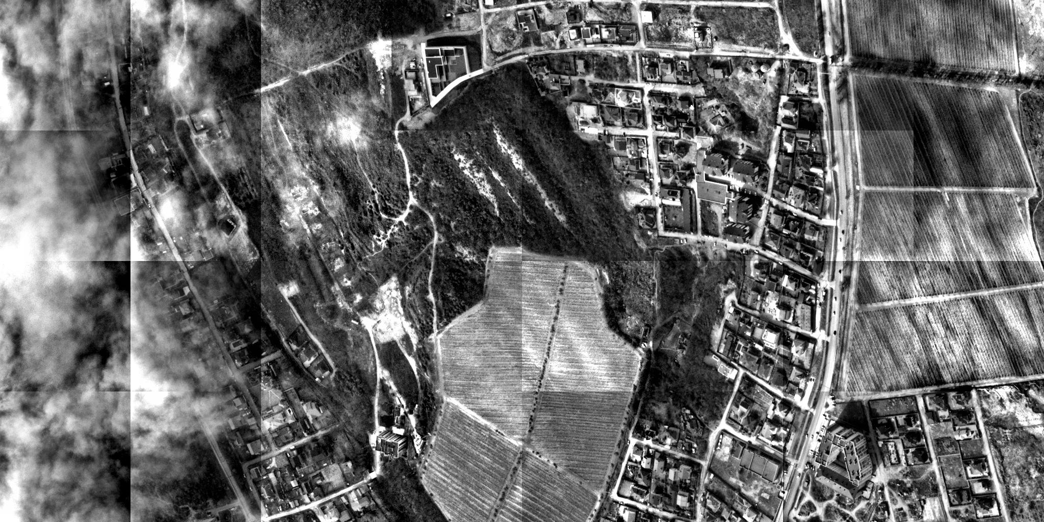
Below, we show the result after chipping the sample image we have previously seen into 512x512 chips and applying a linear stretch and then CLAHE to each chip independently. The apparent checkerboard pattern results from equalization on an individual chip independent of its neighbor. During training or inference, a model would only see a single tile of the checkerboard at a time. Chip size is yet another parameter worth experimenting with. It will impact image quality and model performance in hard-to-predict ways.

Finally, we share some example code to illustrate how chipping and preprocessing can be applied to an image. Note that we use a chip_size that is square (512x512) and assume the input image is much larger than that. Your chips don’t need to be square, but adjustments must be made to this code to accomplish that. We use non-overlapping chips in this example; if you prefer to have overlapping chips, some adjustments to the code are required.

import rasterio
import numpy as np
from PIL import Image
from skimage import exposure

def preprocess(arr):
    # Apply 2% linear stretch and CLAHE to arr, return PIL image.

    lower, upper = np.percentile(arr.flatten(), [2, 98])
    arr = (arr - lower)/(upper - lower)
    arr = np.clip(arr, a_min=0, a_max=1)

    arr = exposure.equalize_adapthist(arr, nbins=256)
    arr = (arr * 255).astype("uint8")

    return Image.fromarray(arr)


src = rasterio.open("/path/to/image.nitf")
arr = src.read(1)
src.close()

max_rows, max_cols = arr.shape
chip_size = 512


# Note: this assumes that max_rows and max_cols are multiples of the chip size
for row in range(0, max_rows, chip_size):
    for col in range(0, max_cols, chip_size):
        # take a slice from row:row+chip_size, col:col+chip_size
        chip_as_array = arr[row:row+chip_size, col:col+chip_size]
        chip_as_pil_img = preprocess(chip_as_array)

        chip_as_pil_img.save("chip-{0}-{1}.png".format(row//512, col//512))