Data Splits

What are data splits?

A data split is a partition of a dataset into several smaller datasets. Typically, a dataset is partitioned (split) into either two or three subsets that are labeled: a training split, a validation split, and a testing split. The resulting partitions of a dataset split thusly serve specific purposes:

• The training split, as its name suggests, is reserved for training (fitting) models.
• The validation split is used to differentiate models (i.e., to determine which model you prefer to deploy).
• The testing split is used one time, only after selecting which (trained) model you will use, and serves the purpose of estimating model performance on unseen, future data.

Why have data splits?

As mentioned above, each of the typical data splits serves a unique purpose. In this section, we describe why one split cannot serve (or shouldn't be made to serve) two purposes.

Why can't training data be used for model validation?

The primary reason, which will be explained in more detail, is that comparing two (or more) models' metrics on training data usually doesn't convey the information that you really want. For example, comparing metrics like "accuracy on training data" (assuming both models' accuracies are not 100%) typically only reflects the relative capacity of a model to learn (models with more parameters generally have more capacity). With extra capacity, models are better able to memorize training examples or model (possibly erroneously) the noise in the data (as if it were signal). And, if training data is used for validation, it makes it nearly impossible to detect overfitting.

Why can't validation data be recycled for testing data?

If data has been used to influence the model (obviously the training data), then that data "has been seen" by the model; hence, using it to estimate accuracy on "unseen" data is, at best, unreliable and, at worst, statistical malpractice. You should always expect metrics that use "seen" data to be overly rosy estimates of performance on "unseen" data. Without actually using "unseen" data, it is (essentially) impossible to know (or estimate) how overly optimistic those estimates of performance are.

But, validation data was not used for training! So, why can't I use it for testing? The answer is: The validation data was subtly used for training. While validation data wasn't directly used to choose the weights/parameter values of models, it did influence the choice of model (which comes with weights/parameter values). So, by examining a number of different models (possibly in various states of training), comparing validation scores, and subsequently choosing the best, you've actually injected yourself (and the validation data) into the training process.

How are data splits constructed?

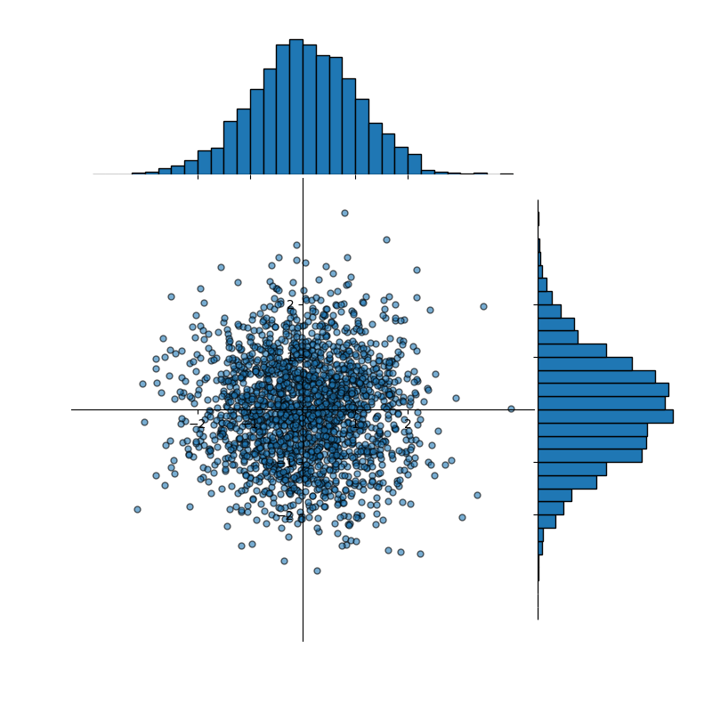
Consider the data shown in Figure 1. The data is sampled from two standard, normal distributions (one for the x-values, and a second for the y-values)—i.e., normal distributions with mean equal to 0 and standard deviation equal to 1. Considering only the x-values of our sample data, the mean and standard deviation are:

$$\mu_x = 0.033, \sigma_x=1.006$$

Considering only the y-values, the data sample has mean and standard deviation are:

$$\mu_y = -0.009, \sigma_y = 0.990$$

Figure 1: A dataset, approximately normally distributed, containing 2,000 data points

In an ideal partitioning of the data into train/test (or train/val, or train/val/test) splits, the essential information of the distribution would be present in each split. In this case, we'd hope that the statistics we compute about the sample training split would be reflected (similarly enough) in the sample testing or sample validation splits (ideally both) and that all three reflect the true underlying distribution that, in this case, we know—but we seldom know in practice. We therefore need to take care to avoid inadvertently biasing one (or all) of the splits. A common way to create the splits in a (usually) unbiased way is to randomly partition the data. There are many ways in which this can be accomplished. Figure 2 shows one such random partitioning. Now our training split (blue) has mean and standard deviation:

$$\mu_{x, blue} = 0.026, \sigma_{x, blue} = 1.011$$ $$\mu_{y, blue} =-0.008, \sigma_{y, blue} = 0.988$$

which is not terribly different than the dataset as a whole. And, the validation (or testing) split (orange) has mean and standard deviation:

$$\mu_{x, orange} = 0.053, \sigma_{x, orange} = 0.988$$ $$\mu_{y, orange} =-0.014, \sigma_{y, orange} = 0.997$$

which is quite similar to both the training data and the dataset as a whole. In other words, both the training and testing data are representative of the dataset as a whole; understanding of the training data translates directly to understanding the dataset as a whole; and measuring results on the testing data will confirm that (because it is so similar to both training data and the dataset as a whole).

Figure 2: A dataset, approximately normally distributed, containing 2,000 data points randomly partitioned into training (blue) and validation (orange) splits

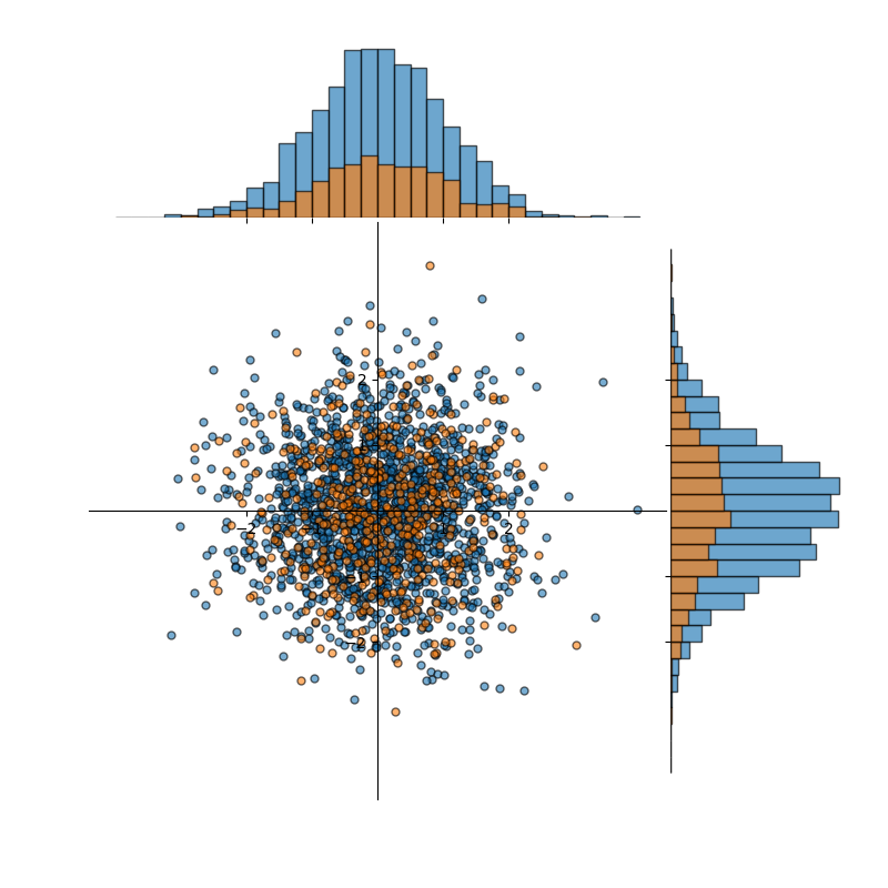
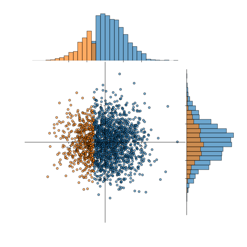
Figure 3 (below) illustrates what can happen if the data is not partitioned well. Note that this illustration is intentionally extreme. However, in practice, it is often significantly harder to detect when datasets are skewed/biased away from reality or when splits of datasets are not taken in a way that preserves distribution characteristics. In this case, our training split (blue) and testing/validation split (orange) agree pretty well with the underlying true distribution when viewing the y-axis only. There we see:

$$\mu_{y,blue} = -0.008, \sigma_{y,blue} = 1.012$$ $$\mu_{y,orange} = -0.011, \sigma_{y,orange}=0.922$$

which is pretty in line with expectations. However, the x-axis is a different story. There we see:

$$\mu_{x,blue} = 0.460, \sigma_{x,blue} = 0.730$$ $$\mu_{x,orange} = -1.247, \sigma_{x,orange} = 0.513.$$

So, not only do the blue and orange distributions differ from each other (viewed along the x-axis), but they also differ significantly from the true underlying distribution.

Figure 3: A dataset, approximately normally distributed, containing 2,000 data points badly partitioned into training and validation splits

Key points to remember when constructing splits

Each of the points below assumes that the dataset you have curated is representative of the true, underlying distribution. If this is not the case, then the quality of your dataset will limit your ability to be effective on unseen data. It will limit your ability to know (estimate) a priori how good or bad your model is, and it will create a host of other challenges. For best possible results, care should be taken when collecting data.

1. Data in splits must be distinct.
   If (some) examples in the training split also appear (as exact duplicates) in the validation or testing split, then those (non-training) splits have become corrupt and are unreliable. In this case, all metrics of goodness will be overly optimistic because you should assume (while it isn't always true, it is frequently enough) that models will be perfectly accurate on training data. As a result, the more overlap there is, the more unreliable the metrics become.

2. Data in splits must be distinct (part 2).
   Whenever possible, it is best to make sure that training splits and any other splits do not contain examples that are too similar (if still technically different). For example, let's consider a dataset of vehicle makes and models. If multiple photos are taken of a single vehicle parked in a single location, but those photos are taken from different angles or with sublty different lighting, then including some in training and some in validation or testing can be problematic. It isn't as bad as having identical images in the two splits; however, it does introduce biases into the data and can have a similarly detrimental effect on metrics (making them unreliable). Anything that increases differences between training data and validation/testing data is good as long as those differences align with the diversity likely to be present in the unseen data. So, back to the vehicle make and model example: If multiple photos of the same car are present, taking those images in different locations is better (than just different angles in a showroom). Likewise, it is better if the ambient conditions are different (maybe sunny, in the dusk/dark, during the rain, etc.).

3. Data in splits must be distinct (part 3).
   Another case where we must (or at least should) pay careful attention is when datasets are obtained by tiling large images. Tiling is the process of cropping a large image
   multiple times to make several (or many) smaller images. To visualize what is happening, imagine a large image being turned into a chess board where each of the 64 tiles (on the 8x8 chessboard) represents a crop of that image—so a single large image is turned into 64 smaller ones. Tiling occurs frequently when working with satellite imagery—for a variety of reasons, not the least of which is the initial image is just too large to process at once. And, there are numerous ways that tiles can be created; crops might overlap, or they might not. In the dataset derived by cropping large images, there are two ways that data may not be completely distinct (or independent). Two non-overlapping tiles from the same original scene (the single large image) might be viewed as independent (distinct); however, they likely have a lot of similarities that are not directly related to the task at hand. For example, the overall brightness of the images will likely be similar (and in most cases, simply comparing brightness is not something you'd want your model to learn); the two crops will likely have similar dynamic ranges (e.g., approximately the same minimum and maximum brightness of individual pixels); and if, for example, one crop is over an urban area, then it's likely the other crop is also over the same urban area (though, likely different neighborhoods), etc. Like before, when we encounter this situation, we have biased the validation or testing data toward the training data in ways that will not likely be reproduced when the model is deployed. Again, the metrics become unreliable (abosutely), and it is difficult to know/estimate the size of the impact—other than that the metrics are likely better than they should be. When the tiling of datasets is overlapped (done for a variety of reasons), including examples from training to testing/validation, that overlap is similarly problematic (likely with a larger impact than that previously mentioned).

Note: Data splits should not be an afterthought. For example, when collecting/curating a dataset, you should already have a plan for partitioning it and take that plan into account when determing how much data needs to be collected. You do not want to be in a position of: "I have to split the datasets thusly because otherwise I don't have sufficient data for X."

Do you always need data splits?

No. There are some (limited) instances when you might not need a data split.

For example, suppose you do not need to select a model from a list of candidate models—e.g., you know your data is linear (with some noise), but you are simply computing a best-fit line. Since the purpose of a validation split is to be able to compare models and since you already know which model is correct, then there is no need for a validation split. However, even in this case, a testing split can be a useful way to estimate future performance on unseen data.

Validation sets (and possibly testing splits) are also not strictly required if you are producing models that do not lend themselves to quantitative evaluation. Examples of such models could be embedding models or autoencoders. Embedding models map a high-dimensional input (e.g., an image) to a low(er)-dimensional "latent" representation. In these cases, it is hard to know what a good embedding looks like—other than the fact that you would hope that similar inputs produce (roughly) similar outputs (e.g., embeddings of cat images should be closer to each other than they are to embeddings of dog images).