Explore Data
Chariot supports various ways to explore the contents of your dataset.
- UI
- SDK
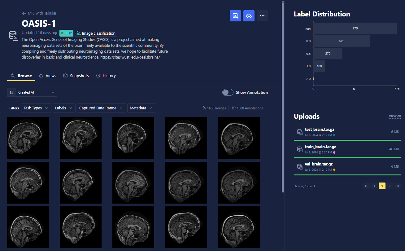
The Browse tab of the Datasets section allows you to view high-level information about the data that populates your dataset. Here, datasets can be easily sorted (from the Sort drop-down) and filtered in order to get an exact view of your specific data. Toggle Show Annotations to show their annotation labels.
On the right, you can view the distribution of annotation labels for the currently applied filter and the history of uploads to your dataset.
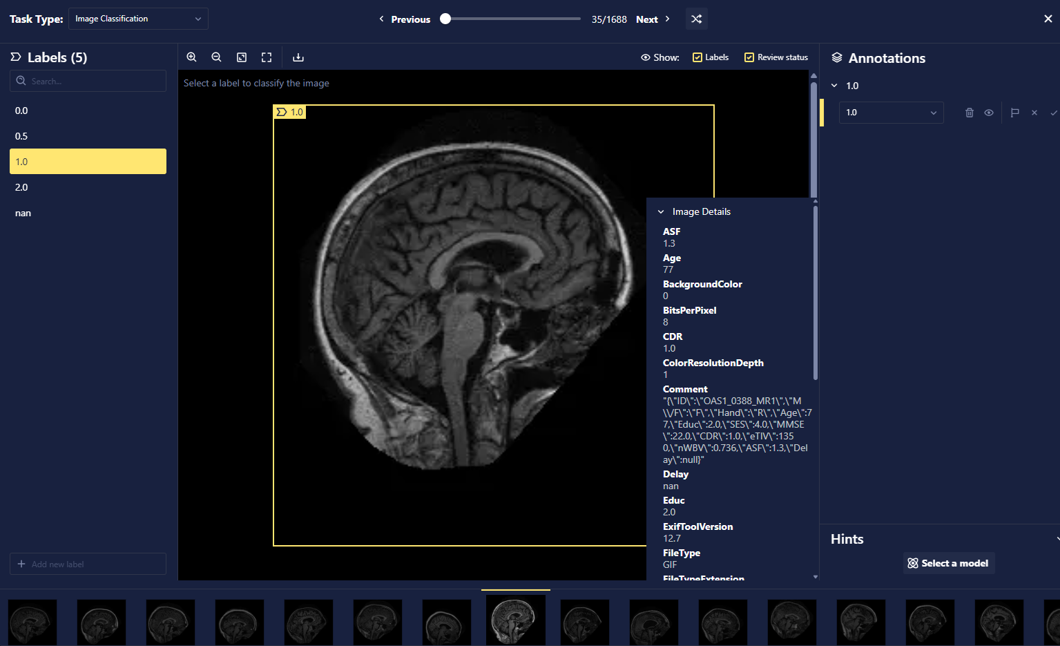
To further inspect a particular data point, which we refer to as a datum, click any of the previews. Metadata about the image can also be viewed from this preview page and used for filtering for specific data.
Filtering
Metadata filters support range-based filtering, allowing you to query for values within specific numeric or date intervals. This makes it easier to isolate records based on properties like file size or timestamp ranges. The system automatically infers the data type of your filter values and applies appropriate comparison logic, with fallback mechanisms for robust querying.
Supported Filter Operations
The following filter operations are supported:
| Operation | UI Representation | Description | Supported Types |
|---|---|---|---|
eq | = equal | Equal to | All types |
neq | != does not equal | Not equal to | All types |
gt | > greater than | Greater than | Numeric, Timestamp, Text |
gte | >= greater than or equal to | Greater than or equal to | Numeric, Timestamp, Text |
lt | < less than | Less than | Numeric, Timestamp, Text |
lte | <= less than or equal to | Less than or equal to | Numeric, Timestamp, Text |
in | ANY of the values from | Any of the specified values | All types (array format) |
full_text | contains text | Performs an English-language full-text search on the metadata value. Matches are case insensitive and word stemming is used (e.g., searching "project" will match "projected"; however, searching "ject" or "poject" will not match "projected" as fuzzy searches are not supported) | Text |
Type Inference and Parsing
The system automatically infers the data type of your filter values using the following priority order:
- Numeric: Attempts to parse as a 64-bit float
- Boolean: Attempts to parse as a boolean (
true/false) - Timestamp: Attempts to parse as a timestamp
- Text: Falls back to lexicographical text comparison
Example: Numeric Fallback
temperature eq "23.5C"- When filtering on this value, numeric parsing fails because of the non-numeric character
C. Instead, lexicographical (text) comparison is used.
- When filtering on this value, numeric parsing fails because of the non-numeric character
Type Inference Examples
temperature eq 23.5→ Inferred as Numeric (23.5)is_processed eq true→ Inferred as Boolean (true)capture_time ≥ 2025-06-01T11:30:15-0700→ Inferred as Timestamp (2025-06-01T18:30:15Z)file_type eq jpeg→ Inferred as Text (jpeg)
Timestamp Format Support
The system supports multiple timestamp formats:
- RFC3339:
2025-06-01T11:30:15Z[Recommended] - With timezone offset:
2025-06-01T11:30:15-0700or2025-06-01T11:30:15+07:00 - DateTime format:
2025-06-01 11:30:15
All timestamps are normalized to UTC for consistent comparison.
Array Values (IN Operation)
For the in operation, provide values as comma separated values:
file_type in "jpeg, png, tiff"
Array Type Inference
Arrays follow the same type inference rules:
- Numeric array:
1, 2, 3.5→ Numeric type - Boolean array:
true, false→ Boolean type - Timestamp array:
"2025-06-01", "2025-06-02"→ Timestamp type - Mixed typesK
true, "yes", 1→ Text type (fallback)
Pitfalls and Best Practices
1. Type Consistency
- Problem: Metadata values are inconsistent.
- Example: Some records have temperature as a number (
23.5), others as a string with units ("23.5C"). - Solution:
- Rely on the fallback behavior that compares both numeric and text.
- Or standardize metadata formats across your dataset for consistency.
2. Timestamp Format Issues
- Problem: Unsupported timestamp formats fallback to lexicographical (text) comparison, causing unexpected filter results.
- Example:
"06012025"is not supported. - Solution: Use supported timestamp formats such as:
2025-06-01T11:30:15Z2025-06-01T11:30:15-07002025-06-01 11:30:15
3. Case Sensitivity
- Problem: Text comparisons are case sensitive.
- Example: Searching for
"JPEG"will not match"jpeg". - Solution:
- Use consistent casing in metadata and filters.
4. Numeric Precision
- Problem: Floating point precision can cause equality filters to fail.
- Example: Filtering for
0.123456789may miss stored values with different decimal places. - Solution:
- Use range filters (e.g., greater than, less than).
- Round values to a suitable precision before filtering.
5. Fraction Not Supported
- Problem: A fraction will not be parsed as a number.
- Example: Filtering for
3/4will only match"3/4", not0.75. - Solution:
- Avoid using fraction as value.
- Or convert fraction values to numbers beforehand.
Troubleshooting
If your metadata filter is not returning the expected results, try the following:
- Check data: Verify the datum metadata is consistent.
- Verify key path: Ensure the key path matches your metadata structure.
- Check for case sensitivity: Text comparisons are case sensitive.
- Validate timestamp format: Use supported timestamp formats.
- Test with simpler filters: Start with basic equality filters to isolate issues.
Using the SDK, users can access datasets, Views, Snapshots, and datums by using a given ID.
from chariot.datasets import get_dataset, get_dataset_views, get_view_snapshots

# Define the dataset ID
dataset_id = "<your_dataset_id>"

dataset = get_dataset(dataset_id)
print(dataset)

views = get_dataset_views(dataset_id)

for view in views:
    snapshots = get_view_snapshots(view.id)
    for snapshot in snapshots:
        print(snapshot)
Dataset(id='2nFjskTT7WwfvSaVebSGXbCYsAA', name='Anti Swim Machines', type=<DatasetType.IMAGE: 'image'>, project_id='2nFc2RAmEWwDILd2xtnOlBA4BYe', is_public=False, is_test=False, delete_lock=True, created_at=datetime.datetime(2024, 10, 10, 15, 58, 45, 746303, tzinfo=tzlocal()), updated_at=datetime.datetime(2024, 10, 10, 16, 1, 38, 41258, tzinfo=tzlocal()), description=None, archived_at=None, archived_by=None, summary=DatasetSummary(datum_count=4000, available_datum_count=0, new_datum_count=0, annotation_count=4054, class_label_count=4000, bounding_box_count=0, oriented_bounding_box_count=54, contour_count=0, text_classification_count=0, token_classification_count=0, text_generation_count=0, class_label_distribution={'not_ship': 3000, 'ship': 1054}, text_classification_distribution=None, token_classification_distribution=None, text_generation_distribution=None, annotation_count_by_approval_status={'': 4054}, total_datum_size=42762748, largest_datum_size=15338, unannotated_datum_count=0), migration_status=None)
Snapshot(id='2vPXEF0jSZaAV4GexqUBOxzwTh6', view=View(task_type_label_filters=[TaskTypeLabelFilter(task_type=<TaskType.IMAGE_CLASSIFICATION: 'Image Classification'>, labels=['not_ship', 'ship'], contexts=None, context_labels=None)], gps_coordinates_circle=None, gps_coordinates_rectangle=None, gps_coordinates_polygon=None, capture_timestamp_range=None, metadata=None, asof_timestamp=None, unannotated=None, datum_ids=None, approval_status=None, annotation_metadata=None, sample_count=None, split_algorithm='random', apply_default_split=True, splits={'test': 0.1, 'train': 0.8, 'val': 0.1}, id='2vPXCVmF0lEYt5uAtOESNhjUKOc', name='Other View', snapshot_count=None, created_at=datetime.datetime(2025, 4, 7, 17, 39, 14, 895667, tzinfo=tzlocal()), updated_at=datetime.datetime(2025, 4, 7, 17, 39, 14, 895667, tzinfo=tzlocal()), archived_at=None, archived_by=None, dataset=Dataset(id='2nFjskTT7WwfvSaVebSGXbCYsAA', name='Anti Swim Machines', type=<DatasetType.IMAGE: 'image'>, project_id='2nFc2RAmEWwDILd2xtnOlBA4BYe', is_public=False, is_test=False, delete_lock=True, created_at=datetime.datetime(2024, 10, 10, 15, 58, 45, 746303, tzinfo=tzlocal()), updated_at=datetime.datetime(2024, 10, 10, 16, 1, 38, 41258, tzinfo=tzlocal()), description=None, archived_at=None, archived_by=None, summary=None, migration_status=None)), name='Other Snapshot', timestamp=datetime.datetime(2024, 10, 10, 15, 59, 57, 992843, tzinfo=tzlocal()), summary=DatasetSummary(datum_count=4000, available_datum_count=0, new_datum_count=0, annotation_count=4000, class_label_count=4000, bounding_box_count=0, oriented_bounding_box_count=0, contour_count=0, text_classification_count=0, token_classification_count=0, text_generation_count=0, class_label_distribution={'not_ship': 3000, 'ship': 1000}, text_classification_distribution=None, token_classification_distribution=None, text_generation_distribution=None, annotation_count_by_approval_status={'': 4000}, total_datum_size=42762748, largest_datum_size=15338, unannotated_datum_count=0), split_summaries={<SplitName.TEST: 'test'>: DatasetSummary(datum_count=400, available_datum_count=0, new_datum_count=0, annotation_count=400, class_label_count=400, bounding_box_count=0, oriented_bounding_box_count=0, contour_count=0, text_classification_count=0, token_classification_count=0, text_generation_count=0, class_label_distribution={'not_ship': 307, 'ship': 93}, text_classification_distribution=None, token_classification_distribution=None, text_generation_distribution=None, annotation_count_by_approval_status={'': 400}, total_datum_size=4262517, largest_datum_size=15338, unannotated_datum_count=0), <SplitName.TRAIN: 'train'>: DatasetSummary(datum_count=3200, available_datum_count=0, new_datum_count=0, annotation_count=3200, class_label_count=3200, bounding_box_count=0, oriented_bounding_box_count=0, contour_count=0, text_classification_count=0, token_classification_count=0, text_generation_count=0, class_label_distribution={'not_ship': 2395, 'ship': 805}, text_classification_distribution=None, token_classification_distribution=None, text_generation_distribution=None, annotation_count_by_approval_status={'': 3200}, total_datum_size=34236590, largest_datum_size=15127, unannotated_datum_count=0), <SplitName.VAL: 'val'>: DatasetSummary(datum_count=400, available_datum_count=0, new_datum_count=0, annotation_count=400, class_label_count=400, bounding_box_count=0, oriented_bounding_box_count=0, contour_count=0, text_classification_count=0, token_classification_count=0, text_generation_count=0, class_label_distribution={'not_ship': 298, 'ship': 102}, text_classification_distribution=None, token_classification_distribution=None, text_generation_distribution=None, annotation_count_by_approval_status={'': 400}, total_datum_size=4263641, largest_datum_size=15070, unannotated_datum_count=0)}, status=<SnapshotStatus.COMPLETE: 'complete'>, created_at=datetime.datetime(2025, 4, 7, 17, 39, 27, 631229, tzinfo=tzlocal()), updated_at=datetime.datetime(2025, 4, 7, 17, 39, 27, 631229, tzinfo=tzlocal()))
We can then use common Python libraries such as pandas and Matplotlib for further exploration of the data. In the following example, we will use the SDK to get the metadata of all the individual datums in the dataset, load it into a pandas DataFrame, and do some analysis.
import pandas as pd
import matplotlib.pyplot as plt
from chariot.datasets import get_dataset_datums
dataset_id = "<your_dataset_id>"
# Fetch datums
datums = get_dataset_datums(dataset_id)
# Initialize a list to store the extracted data
data = []
# Iterate over the datums and extract the desired fields
for datum in datums:
datum_id = datum.id
class_label = datum.annotations[0].class_label if datum.annotations else None
metadata = datum.metadata
# Flatten metadata dictionary
metadata_flat = {'datum_id': datum_id, 'class_label': class_label}
metadata_flat.update(metadata)
# Append the flattened metadata to the data list
data.append(metadata_flat)
# Create a pandas DataFrame from the data list
df = pd.DataFrame(data)
# Remove duplicates based on patient ID
df_unique = df.drop_duplicates(subset=['ID'])
# Convert Educ, Age, and class_label to numeric values
df_unique['Educ'] = pd.to_numeric(df_unique['Educ'], errors='coerce')
df_unique['Age'] = pd.to_numeric(df_unique['Age'], errors='coerce')
df_unique['class_label'] = pd.to_numeric(df_unique['class_label'], errors='coerce')
# Compute distributions
distributions = {
'M/F': df_unique['M/F'].value_counts(normalize=True),
'Age': df_unique['Age'].describe(),
'Educ': df_unique['Educ'].describe()
}
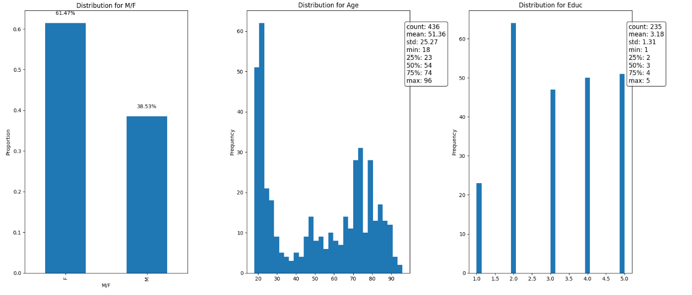
# Plot distributions
fig, axs = plt.subplots(1, 3, figsize=(18, 6))
# Plot M/F distribution
distributions['M/F'].plot(kind='bar', ax=axs[0], title='Distribution for M/F')
axs[0].set_ylabel('Proportion')
for i, v in enumerate(distributions['M/F']):
axs[0].text(i, v + 0.02, f"{v:.2%}", ha='center')
# Plot Age distribution
df_unique['Age'].plot(kind='hist', bins=30, ax=axs[1], title='Distribution for Age')
axs[1].set_ylabel('Frequency')
stats_age = distributions['Age']
axs[1].text(0.98, 0.95, f"count: {stats_age['count']:.0f}\nmean: {stats_age['mean']:.2f}\nstd: {stats_age['std']:.2f}\nmin: {stats_age['min']:.0f}\n25%: {stats_age['25%']:.0f}\n50%: {stats_age['50%']:.0f}\n75%: {stats_age['75%']:.0f}\nmax: {stats_age['max']:.0f}",
transform=axs[1].transAxes, fontsize=12, verticalalignment='top', bbox=dict(boxstyle='round', facecolor='white', alpha=0.8))
# Plot Educ distribution
df_unique['Educ'].plot(kind='hist', bins=30, ax=axs[2], title='Distribution for Educ')
axs[2].set_ylabel('Frequency')
stats_educ = distributions['Educ']
axs[2].text(0.98, 0.95, f"count: {stats_educ['count']:.0f}\nmean: {stats_educ['mean']:.2f}\nstd: {stats_educ['std']:.2f}\nmin: {stats_educ['min']:.0f}\n25%: {stats_educ['25%']:.0f}\n50%: {stats_educ['50%']:.0f}\n75%: {stats_educ['75%']:.0f}\nmax: {stats_educ['max']:.0f}",
transform=axs[2].transAxes, fontsize=12, verticalalignment='top', bbox=dict(boxstyle='round', facecolor='white', alpha=0.8))
plt.tight_layout()
plt.show()
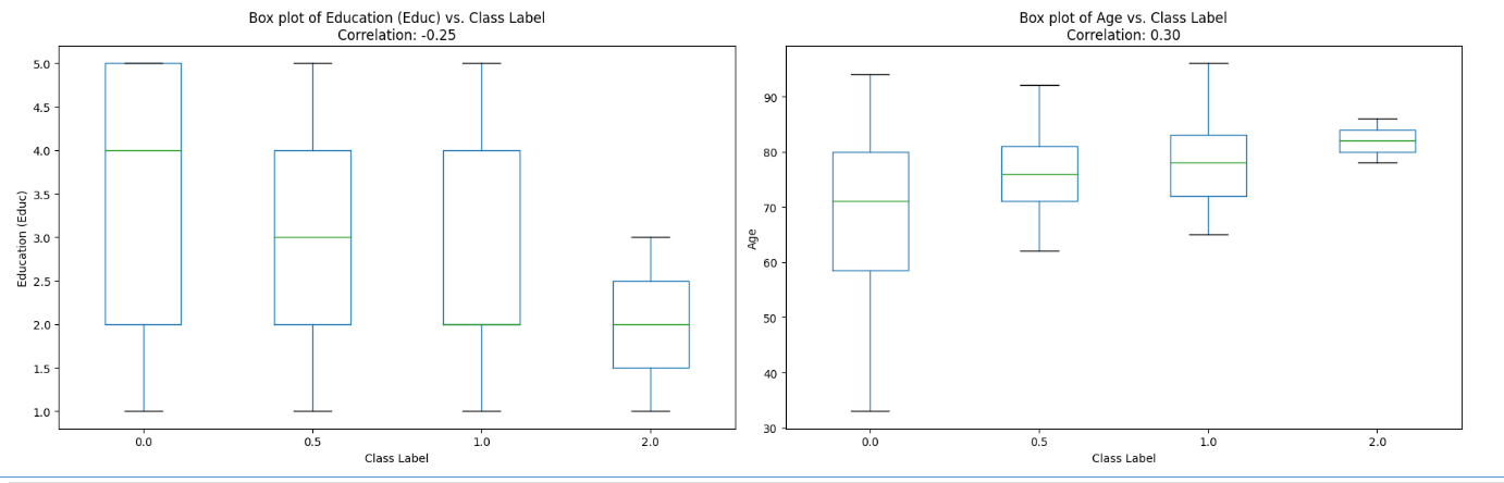
# Calculate correlation for Educ and Age with class_label
correlation_educ = df_unique[['Educ', 'class_label']].corr().iloc[0, 1]
correlation_age = df_unique[['Age', 'class_label']].corr().iloc[0, 1]
# Plot box plots on a separate row
fig, axs = plt.subplots(1, 2, figsize=(18, 6))
# Box plot for Educ vs. class_label
df_unique.boxplot(column='Educ', by='class_label', grid=False, ax=axs[0])
axs[0].set_title(f'Box plot of Education (Educ) vs. Class Label\nCorrelation: {correlation_educ:.2f}')
axs[0].set_xlabel('Class Label')
axs[0].set_ylabel('Education (Educ)')
axs[0].figure.suptitle('')
# Box plot for Age vs. class_label
df_unique.boxplot(column='Age', by='class_label', grid=False, ax=axs[1])
axs[1].set_title(f'Box plot of Age vs. Class Label\nCorrelation: {correlation_age:.2f}')
axs[1].set_xlabel('Class Label')
axs[1].set_ylabel('Age')
axs[1].figure.suptitle('')
plt.tight_layout()
plt.show()